Screening Tests, Predictive Values, and Study Results
Build screening metrics from patient counts, update disease odds, assess screening benefit, and interpret risk reductions, study designs, and uncertainty.
A test can detect 95% of people with a disease while most positive results in a screening clinic are false positives. Those statements answer different questions. Start by naming the group in the denominator, then ask how much the result changes this patient's probability and whether acting on it improves outcomes.
First decide whether you know disease status from a reference standard, the test result, or both. A positive screen is not itself a diagnosis.
Four cells tell you which question was answered
Imagine 1,000 people tested with a defined reference standard. One hundred have the target condition and 900 do not. The new test detects 90 of the 100 affected people and labels 80 unaffected people positive. These are illustrative counts, not performance claims about a named clinical assay.
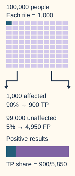
Open whole imageCount from the population into the positive-result group. Teaching assumptions are prevalence 1%, sensitivity 90%, specificity 95%. Tile colors identify reference status; strip colors identify true versus false positive results.Image: Bone Wizardry original mathematical illustration, assistant-authored. Original artwork; no third-party license asserted. Original source.
Reference status determines the columns; the new test determines the rows
New test
Condition present
Condition absent
New testPositive
Condition present90 true positives
Condition absent80 false positives
New testNegative
Condition present10 false negatives
Condition absent820 true negatives
Read down a condition column for sensitivity or specificity. Read across a result row for a predictive value.
Sensitivity is TP/(TP + FN). Here it is 90/100, or 90%. Its complement is the false-negative rate among people with the condition. Specificity is TN/(TN + FP). Here it is 820/900, about 91.1%. Its complement is the false-positive rate among people without the condition. A 5% false-negative rate is not a 5% probability of disease after a negative result. Those denominators differ. [1]
Positive predictive value is TP/(TP + FP). Here 90/170, or 52.9%, of positive results are true positives. Negative predictive value is TN/(TN + FN). Here 820/830, or 98.8%, of negative results are true negatives. Prevalence is 100/1,000, or 10%. Accuracy is (TP + TN)/total, here 91%. Accuracy alone can mislead when one condition status dominates the sample. A test that always says negative can look highly accurate in a population where disease is rare.
These calculations assume reference status is established appropriately. Comparing two imperfect tests establishes agreement, not automatically sensitivity and specificity. Verifying only positive screens can distort accuracy estimates because disease among negative screens is not assessed comparably. When complete verification is impractical, use a justified probability sample with known sampling probabilities, the same appropriate reference standard, and estimation adjusted for the sampling design. Prespecification alone does not make a sample representative. Include relevant patient subgroups, account for indeterminate results, and report uncertainty around performance estimates. [1]
Try it here · Checkpoint 1 of 3
Make your prediction before reading the choices. A first attempt is just a starting point.
Case 2
Show answer and explanations for case 2
A. 92% specificity; reference-verify probability samples from all cells and apply sampling weights (Why this does not fit)
Read the complete explanation
The verification design is useful, but comparator-negative people are not known to be truly disease-free. Thus 460/500 is not specificity.
B. 92% negative percent agreement; reference-verify only discordant cells and estimate accuracy from those results (Why this does not fit)
Read the complete explanation
The agreement label is right, but disease status among 550 concordant results remains unknown. Discordance-only adjudication cannot identify accuracy.
C. 92% specificity; reference-verify only discordant cells and estimate accuracy from those results (Why this does not fit)
Read the complete explanation
Neither the imperfect comparator identifies true negatives nor discordance-only verification covers the agreement cells.
D. 92% negative percent agreement; reference-verify probability samples from all cells and apply sampling weights (Best answer)
Read the complete explanation
The denominator is comparator negatives, so 460/500 is negative percent agreement. Reference verification across all cells with known selection probabilities permits design-adjusted accuracy estimates.
Takeaway: Comparator agreement is not accuracy; reference verification needs coverage of concordant and discordant cells.
The same result means different things in different populations
Holding sensitivity and specificity fixed, increasing prevalence raises PPV and lowers NPV. The fixed-performance assumption is a calculation condition, not a promise that test performance never changes between settings. Disease severity, competing diagnoses, specimen collection, timing, and the reference standard can change observed sensitivity and specificity. A validation sample containing only severe disease and very healthy controls can overstate performance in ordinary patients. This is spectrum bias. [1]
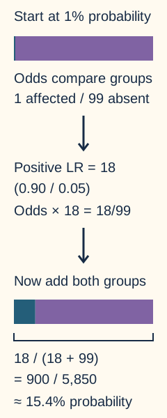
Open whole imageThe positive likelihood ratio multiplies odds, not probability. Strip widths show disease and no-disease proportions. Count units change from 1/99 to 18/99; the matching cohort ratio is 900/4,950. These are illustrative calculations, not real-assay performance.Image: Bone Wizardry original mathematical illustration, assistant-authored. Original artwork; no third-party license asserted. Original source.Natural frequencies for a 95% sensitive, 95% specific test in 10,000 people
A larger affected group supplies more true positives. The large unaffected group at low prevalence supplies many false positives even with good specificity.
Worked cohort, without a calculator: In 100,000 people at 1% prevalence, an illustrative test with 90% sensitivity and 95% specificity yields 900 true positives, 4,950 false positives, 100 false negatives, and 94,050 true negatives. Among 5,850 positive results, 900 represent disease. At 20% prevalence with the same operating point, the four counts are 18,000, 4,000, 2,000, and 76,000, so 18,000 of 22,000 positives represent disease. At 1% prevalence, a different illustrative lower cutoff with 98% sensitivity and 80% specificity yields 980, 19,800, 20, and 79,200. These are teaching assumptions, not measurements of a real assay. [1]
For an individual, use the relevant pretest probability, informed by the population and clinical findings. Likelihood ratios provide an odds update. LR+ = sensitivity/(1 − specificity). LR− = (1 − sensitivity)/specificity. Convert probability p to odds p/(1 − p), multiply by the LR for the observed result, then convert odds o back to probability o/(1 + o).
At 10% pretest probability, odds are 1/9. A positive result with LR+ 12 gives odds 12/9 and probability 57.1%. At 80% pretest probability, odds are 4. A negative result with LR− 0.05 gives odds 0.20 and probability 16.7%. Even a strong negative likelihood ratio leaves substantial residual probability when the starting probability is high. Likelihood ratios multiply odds, not probabilities. [1][24]
SnNOut and SpPIn are reminders about favorable test characteristics, not stand-alone clinical verdicts. Whether a result crosses a testing or treatment threshold depends on the full performance, pretest probability, and consequences of error. For example, current CDC guidance calls for backup throat culture after a negative rapid antigen detection test in symptomatic children aged three years or older. A reassuring mnemonic does not replace that specific testing pathway. [11]
Try it here · Checkpoint 2 of 3
Make your prediction before reading the choices. A first attempt is just a starting point.
Case 8
Show answer and explanations for case 8
A. Arrange follow-up only if symptoms persist, without culture now (Why this does not fit)
Read the complete explanation
Symptom follow-up is useful, but it does not replace the recommended backup culture after negative RADT in this age group.
B. Repeat RADT tomorrow and treat if that repeat is positive (Why this does not fit)
Read the complete explanation
A repeat antigen test is not the CDC-specified backup throat culture for this symptomatic child.
C. Start antibiotics now and culture only if symptoms persist (Why this does not fit)
Read the complete explanation
Compatible symptoms are insufficient to confirm GAS; backup culture should be obtained rather than empirical treatment after the negative RADT.
D. Obtain backup throat culture and follow its result (Best answer)
Read the complete explanation
A symptomatic child older than three with negative RADT needs backup culture; the contact system enables follow-up if positive.
Takeaway: Negative RADT in symptomatic children aged three or older needs backup culture.
A cutoff changes classification, not the underlying measurements
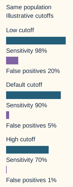
For a test where higher values indicate disease, lowering the positivity threshold labels more results positive. Sensitivity cannot decrease and specificity cannot increase in the same dataset. Some cutoff changes produce no change if no observations lie between them. Raising the threshold has the opposite direction. If lower values indicate disease, reverse the numerical direction of the cutoff rule.
Open whole imageDark bars use affected people as their denominator. Purple bars use unaffected people. All bars use a zero-to-100% scale. Raising the illustrative cutoff reduces detection and false positives; it does not change prevalence.Image: Bone Wizardry original mathematical illustration, assistant-authored. Original artwork; no third-party license asserted. Original source.
The ROC curve plots sensitivity against the false-positive rate, 1 − specificity, across cutoffs. The upper-left region combines high sensitivity with few false positives. ROC area under the curve summarizes discrimination across thresholds. An AUC of 0.5 indicates no rank discrimination and 1 indicates perfect rank discrimination in the evaluated population; values below 0.5 are possible, for example when score direction is reversed. AUC is not PPV, accuracy at one cutoff, calibration, or proof of clinical benefit. [1]
Precision-recall displays answer a related question using PPV, also called precision, against sensitivity, also called recall. Because PPV changes with prevalence, interpret these plots in the evaluated population. Neither an appealing curve nor a statistically selected balance of sensitivity and specificity determines the best clinical threshold. Missed disease, false-positive procedures, treatment effects, and resource use must be considered.
Screening often places substantial weight on sensitivity, but false positives are not harmless. A diagnostic pathway may use subsequent testing to improve certainty, yet repeated tests are not automatically independent. Do not multiply likelihood ratios for correlated tests without a justified model. Check what outcome defines disease, what threshold defines a positive screen, and what subsequent action is supported.
Finding disease earlier is not the same as improving health
Lead-time bias changes the starting date. In a hypothetical example, symptom diagnosis occurs at age 66 and death at 70. Screening diagnoses the same disease at 63 without changing death at 70. Survival from diagnosis grows from four to seven years while lifespan is unchanged. This arithmetic example does not assert that a particular screening program lacks benefit.
Length-time bias changes which disease is detected. A slowly progressing tumor remains detectable before symptoms for longer, so periodic screening is more likely to find it. Aggressive tumors may become symptomatic between screens. The screen-detected group can therefore have more favorable biology independent of screening benefit. Overdiagnosis identifies a real condition that would never have caused symptoms or death during the person's lifetime. It is distinct from a false-positive result. [2]
A randomized screening comparison with appropriate mortality follow-up in the entire assigned population addresses these interpretive traps more directly than comparing survival only among diagnosed cases. Disease-specific mortality is informative, with careful cause-of-death assessment; all-cause mortality and harms provide complementary information. Randomization does not make screen-detected tumors representative of all tumors, and it does not erase missed follow-up, contamination, or other study limitations.
Evaluate the complete program. Benefits depend on whether earlier detection permits effective action; harms include false-positive workup and unnecessary treatment of overdiagnosed disease. A high detection count, small average tumor size, or improved survival from diagnosis is insufficient by itself to establish net benefit. [2]
Read the absolute difference and its uncertainty
For an adverse event, absolute risk reduction is control risk minus treatment risk. Relative risk is treatment risk divided by control risk, and relative risk reduction is 1 − RR. If five-year event risks are 8% and 4%, ARR is four percentage points, RR is 0.5, RRR is 50%, and NNT is 1/0.04 = 25 over five years. For a positive noninteger NNT, round upward to a whole patient for conventional reporting. The time horizon, outcome, comparator, and population belong with the number. [4][23]
For harm, absolute risk increase is treatment risk minus comparison risk and NNH is its reciprocal. An NNH of 50 over one year corresponds to two additional events per 100 treated over that year, not a total adverse-event rate of 2% or 50%. NNT and NNH are average comparative summaries. They neither identify which individual benefits nor show that every other patient receives no benefit of any kind.
Comparing their numerical sizes alone cannot weigh a mild benefit against a severe harm. Use comparable follow-up periods and an explicit valuation or resource rule when a decision requires trading benefit against harm. [23]
A p value describes how incompatible the observed result is with a specified null model using the chosen test statistic. It is not the probability that the null is true, that the result is a mistake, or that treatment works. Statistical significance does not establish clinical importance or freedom from bias. A small blood-pressure difference may matter differently by risk, cost, harms, and duration; there is no universal minimum useful change implied by p. [5]
A confidence interval shows estimation uncertainty under the method's assumptions. For matched two-sided methods, a 95% interval excluding the null corresponds to rejection at alpha 0.05. The null is 1 for ratios and 0 for differences. A frequentist 95% confidence procedure covers the fixed true parameter in 95% of repeated applications under its assumptions. An interval including the null does not prove equivalence. Equivalence requires excluding effects beyond both prespecified margins; noninferiority excludes unacceptable inferiority on one specified side. [3][10]
Type I error rejects a true null. Type II error fails to reject a false null. Power is 1 − beta for a specified alternative and design. More participants or less measurement noise generally improves power, holding other conditions fixed. A nonsignificant small study may be imprecise; its result alone cannot establish that a Type II error actually occurred.
Try it here · Checkpoint 3 of 3
Make your prediction before reading the choices. A first attempt is just a starting point.
Case 17
Show answer and explanations for case 17
A. The 25% is the overall relative risk reduction, not the one-percentage-point absolute reduction; the subgroup results do not establish a difference in relative effects (Best answer)
Read the complete explanation
Overall risk ratio is 3/4 = 0.75, so relative reduction is 25% and absolute reduction is 1 percentage point. The subgroup CI includes 1 and interaction p = 0.60 provides no evidence of different effects, not proof of equality.
B. The 25% is the overall relative risk reduction; the nonsignificant subgroup result establishes a smaller relative benefit there (Why this does not fit)
Read the complete explanation
The overall relative reduction is 25%. A nonsignificant result within one subgroup cannot establish that its effect is smaller than another subgroup effect; the interaction p = 0.60 does not show a difference.
C. The 25% is the overall absolute risk reduction; the subgroup results do not establish a difference in relative effects (Why this does not fit)
Read the complete explanation
The absolute reduction is 4% - 3% = 1 percentage point, not 25%; 25% divides that difference by the 4% control risk.
D. The 25% is the overall relative risk reduction; the nonsignificant interaction establishes equal relative effects (Why this does not fit)
Read the complete explanation
The overall relative reduction is 25%. Interaction p = 0.60 does not establish equality of subgroup effects.
Takeaway: An overall relative reduction differs from the absolute reduction; within-subgroup nonsignificance does not demonstrate effect modification.
An RCT assigns interventions randomly. A cohort follows an exposure-defined population through outcome time, prospectively or using records, and can estimate risks. A conventional case-control study samples by outcome and compares prior exposures, usually using an odds ratio without directly estimating population incidence. Cross-sectional studies measure a population at a point or period and often estimate prevalence. Case series lack a comparison group but can identify signals worth investigating. Matching controls is optional, not definitional. [18][3]
For independent categorical counts, chi-square uses expected cell counts; sparse 2 by 2 tables often favor Fisher exact. Expected counts are row total times column total divided by the grand total; they are not the observed counts. [22] For two independent continuous means, use an appropriate t procedure, often Welch when variances need not be equal.
Paired t tests use within-person differences. One-way ANOVA compares independent group means under its assumptions; significant omnibus evidence does not identify which pairs differ. Specific contrasts need an appropriate prespecified analysis with multiplicity control when several claims form a family. A significant omnibus test is not a universal prerequisite for a prespecified contrast. Bonferroni intervals allocate alpha across a finite planned family to control simultaneous coverage. [19][20][12][13][14]
Mann-Whitney compares ranks in two independent samples. When the distributions differ only by a location shift, that difference can be described as a difference in medians; different shapes make a median-only reading inadequate. [15] Kruskal-Wallis compares rank sums across independent groups under a common-distribution null. Rejection does not by itself establish a median difference or identify the differing pairs. [17][21] Pearson correlation describes linear association of measured values; Spearman describes association of their ranks and can capture monotonic relationships. Neither establishes causation or measurement agreement. Paired, repeated, clustered, or censored data need methods respecting those structures. [15][16]
Bias may enter through recruitment, recall, outcome assessment, treatment selection, or missing outcomes. Hospital admission can distort associations when it depends on both exposure and disease, the Berkson mechanism. Awareness of observation can alter behavior, the Hawthorne effect, without necessarily inflating a between-group effect. Intention-to-treat preserves original assignment but cannot recover unobserved outcomes without assumptions. There is no universally safe dropout percentage. [3][6]
In evidence synthesis, forest plots display estimates and intervals; a pooled result inherits the limitations of its studies. I-squared is not a rule that automatically prohibits pooling above 50%. Funnel asymmetry can arise from missing evidence, heterogeneity, methodological differences, or chance. Prespecified interim monitoring can support ethical early stopping, but repeated examination and effect estimation require appropriate statistical control. [7][8][9]
The bias and study-design lesson develops recruitment, confounding, trial follow-up and evidence synthesis in more detail.
Name the denominator, update the odds, identify the design, inspect absolute effects and uncertainty, then decide what clinical action the evidence supports.
When assignment changes treatment uptake, the effect of assignment and the effect of receiving treatment are different questions. With random assignment, an exclusion restriction, no defiers and a nonzero uptake difference, divide the assignment outcome contrast by the uptake contrast. This Wald ratio estimates the effect among people whose uptake changes with assignment, not automatically the whole population. [27]
Practice interpreting tests and study results
Case 1
Show answer and explanations for case 1
A. 90% in this advanced-disease validation setting; obtain evidence in the intended early-disease spectrum (Best answer)
Read the complete explanation
The five verified false negatives represent ten after weighting, so 90/(90+10) = 90%. Advanced-only disease validation cannot establish early-disease sensitivity.
B. 94.7% in this validation setting; obtain evidence in the intended early-disease spectrum (Why this does not fit)
Read the complete explanation
Five is only the sampled false-negative count. The random half-sample represents ten false negatives before estimating sensitivity.
C. 90% here; apply it unchanged to early-disease screening (Why this does not fit)
Read the complete explanation
The weighting gives 90%, but the validation contains no diseased patients with early disease. Its sensitivity may not transport.
D. 94.7% here; apply it unchanged to early-disease screening (Why this does not fit)
Read the complete explanation
This uses the unweighted five false negatives and also transports an advanced-only estimate to an unstudied spectrum.
Takeaway: Verification weighting corrects the sampled result stratum; disease spectrum limits transport.
A. 81.82% in the selected sample; use it in the clinic after checking that the same assay threshold is used (Why this does not fit)
Read the complete explanation
The threshold alone does not transport predictive value: deliberate 50% prevalence differs from the 2% clinic, and disease severity also differs.
B. 90% in the selected sample; measure clinic prevalence and performance in its disease spectrum (Why this does not fit)
Read the complete explanation
The additional evidence is appropriate, but 90% is specificity, 90/(90+10), not NPV among negative tests.
C. 81.82% in the selected sample; obtain accuracy in the intended severity spectrum and representative clinic prevalence before a clinic rule-out estimate (Best answer)
Read the complete explanation
The selected-sample negative results give 90/(90+20). Neither its predictive value nor advanced-disease sensitivity transports to mostly mild disease; clinic prevalence is also needed.
D. 81.82% in the selected sample; combine its 80% sensitivity and 90% specificity with 2% prevalence without further accuracy evidence (Why this does not fit)
Read the complete explanation
Clinic prevalence alone is insufficient: advanced-only validation does not establish mild-disease sensitivity at this threshold.
Takeaway: Selected case-control predictive values and advanced-disease accuracy do not establish mild-disease clinic NPV.
A. Positive results are more reliable in B (92.31% versus 66.67%) because current prevalence is higher; B also has higher infection incidence (Why this does not fit)
Read the complete explanation
PPV and current prevalence are correctly inferred, but a one-visit table has no new-case onset rate or person-time.
B. Both PPVs are 90% because sensitivity is the same; infection incidence cannot be compared (Why this does not fit)
Read the complete explanation
The incidence caution is sound, but 90% conditions on disease, not positive results; false-positive counts differ.
C. Positive results are more reliable in B (92.31% versus 66.67%) with greater current prevalence despite matched accuracy; incidence is not identified (Best answer)
Read the complete explanation
PPVs are 360/390 and 90/135. Both sensitivities are 90% and specificities 95%; these one-visit data do not give incident onsets.
D. Positive results are more reliable in B (92.31% versus 66.67%) because its sensitivity is higher; incidence is not identified (Why this does not fit)
Read the complete explanation
The PPV and incidence conclusion fit, but B sensitivity is 360/400 = 90%, equal to A 90/100. Current prevalence differs.
Takeaway: Current prevalence can change PPV without revealing incidence.
A. A despite its lower 50% sensitivity at 2% false positives; about 40% clinic PPV (Why this does not fit)
Read the complete explanation
A has larger global AUC, but B detects 65% rather than 50% at the clinic false-positive constraint. The roughly 40% projection pertains to B, not A.
B. A despite its lower local sensitivity; about 97% PPV from the 1:1 sample (Why this does not fit)
Read the complete explanation
A has lower sensitivity at 2% false positives, and the 1:1 predictive value cannot be carried to 2% prevalence.
C. B for 65% versus 50% sensitivity at 2% false positives; about 97% clinic PPV (Why this does not fit)
Read the complete explanation
B is the right local choice, but 97.01% conditions on the validation sample with 50% disease prevalence.
D. B for 65% versus 50% sensitivity at 2% false positives; about 39.88% projected clinic PPV (Best answer)
Read the complete explanation
B wins at the constrained operating point despite lower AUC. With assumed transport, (.65*.02)/(.65*.02+.02*.98) = 39.88%, not the 1:1 sample PPV.
Takeaway: Monotone piecewise-linear vertices make both same-cohort ROC summaries feasible. Local performance and projected PPV answer different questions; descriptive AUCs alone do not establish population superiority.
A. Reference-test a random subset of negatives but calculate sensitivity only among all verified patients without adjustment (Why this does not fit)
Read the complete explanation
The negative sample can reveal false negatives, but the raw verified subset overrepresents positives because all positives versus only some negatives were verified.
B. Reference-test a random subset of negatives with known sampling probabilities, then weight by those probabilities (Best answer)
Read the complete explanation
Random negative verification using the same reference standard reveals otherwise unobserved false negatives; design-weighted estimation accounts for unequal verification.
C. Repeat the index assay in a random subset of negatives and use inverse-probability weighting (Why this does not fit)
Read the complete explanation
Random sampling and weights do not solve the absence of disease status if the same index assay is repeated instead of an appropriate reference standard.
D. Reference-test the first 100 negatives and weight each as nine negatives (Why this does not fit)
Read the complete explanation
A fixed first 100 are not a known-probability random sample of the 900; weighting cannot remove order-dependent selection bias.
Takeaway: Partial verification can support adjusted accuracy estimates when sampling is known.
A. Survival rises from 4 to 7 years but neither pathway crosses the five-year mark (Why this does not fit)
Read the complete explanation
The no-screen four-year interval does not cross five years; the screen-diagnosed seven-year interval does.
B. Survival remains 4 years in both pathways because age at death is unchanged (Why this does not fit)
Read the complete explanation
The unchanged death age does not fix diagnosis-to-death time when diagnosis shifts three years earlier.
C. Survival rises from 4 to 7 years and crosses the five-year mark, implying three additional life-years (Why this does not fit)
Read the complete explanation
The survival durations and threshold crossing are right, but the death age is 70 in both pathways, so the three added measured years are lead time.
D. Survival rises from 4 to 7 years and crosses the five-year mark, while age at death is unchanged (Best answer)
Read the complete explanation
Diagnosis-to-death duration is 70 - 66 = 4 versus 70 - 63 = 7 years; death remains at 70, so apparent five-year survival improves without life extension.
Takeaway: Lead time can change diagnosis-anchored survival without changing death time.
A. About 80% slow; longer diagnosed-case survival establishes a screening treatment effect (Why this does not fit)
Read the complete explanation
The 4:1 detection ratio is right, but enrichment of slower disease can explain favorable case survival without an intervention effect.
B. About 50% slow; longer diagnosed-case survival could reflect duration selection (Why this does not fit)
Read the complete explanation
Equal incidence is not equal representation after annual sampling: slow tumors are seen with probability 1, aggressive with .25.
C. About 94% slow; longer diagnosed-case survival could reflect duration selection (Why this does not fit)
Read the complete explanation
Dividing raw windows, four years/.25 years = 16:1 (94.1%), ignores saturation: the slow detection probability is capped at 1 over annual visits.
D. About 80% slow; longer diagnosed-case survival could reflect duration selection (Best answer)
Read the complete explanation
A four-year window guarantees at least one annual screen, whereas three months gives 3/12 = 25% chance. Equal onset gives slow:aggressive detection 1:.25 = 4:1, or 80% slow; selection can lengthen observed survival.
A. The remaining 50 diagnoses could include overdiagnosis or later presentations; treatment adds measured harm (Best answer)
Read the complete explanation
At year 15, 200 - 150 = 50 extra real diagnoses remain after partial catch-up. This is compatible with overdiagnosis as a contributor, but delayed cases and uncertainties prevent labeling any one lesion; treatment complications matter.
B. The 80-diagnosis early excess is fully explained by advancing diagnosis, since the control group partially catches up (Why this does not fit)
Read the complete explanation
At year 5 the gap is 180 - 100 = 80; at year 15 it narrows but remains 200 - 150 = 50, so pure completed catch-up does not account for all diagnoses under this follow-up.
C. The remaining 50-diagnosis excess estimates 50 people harmed by treatment during follow-up (Why this does not fit)
Read the complete explanation
The incidence difference is 50, but it is not a count of treatment complications or a certain classification of individual overdiagnoses; harm requires its own outcome data.
D. The excess is best counted as 50 false-positive pathology reports because mortality is unchanged (Why this does not fit)
Read the complete explanation
The excess counts pathologically confirmed diagnoses, not false-positive test results; unchanged mortality alone does not classify the pathology.
Takeaway: Persistent excess of real diagnoses with incomplete catch-up can support overdiagnosis without proving each case.
A. Screening prevents about 20 disease deaths but causes about 60 extra complications, a net loss of 40 lives per 10,000 (Why this does not fit)
Read the complete explanation
Both absolute differences are correct, but a serious workup complication is not automatically equivalent to a death; subtracting counts as lives is invalid.
B. Per 10,000 invited: 20 fewer disease deaths and 60 extra serious complications; value the outcomes separately (Best answer)
Read the complete explanation
The assigned-group differences are 60 - 40 = 20 fewer disease deaths and 90 - 30 = 60 extra serious complications per 10,000. Their counts cannot be simply netted as equal outcomes.
C. Screening prevents about 60 disease deaths and causes about 60 extra complications per 10,000 invited (Why this does not fit)
Read the complete explanation
Sixty is the usual-care disease-death count, not the reduction; the reduction is 20.
D. Screening prevents about 20 disease deaths and causes about 90 extra serious complications per 10,000 invited (Why this does not fit)
Read the complete explanation
The mortality difference is correct; 90 is total complications in screening, not the excess over 30 in usual care, which is 60.
Takeaway: Compare mortality benefit and diagnostic harms on the same randomized denominator without treating unlike outcomes as interchangeable.
A. NNT 50 and NNH 100 over two years in eligible trial patients; bleeding risk for the excluded anticoagulant regimen needs separate evidence (Best answer)
Read the complete explanation
Event risk falls from 100/1000 to 80/1000, an absolute 2% reduction (NNT 50). Bleeding rises from 40/1000 to 50/1000, an absolute 1% increase (NNH 100). Exclusion leaves the anticoagulant interaction unknown.
B. NNT 50 and NNH 100 over two years; use NNH 100 as the anticoagulated patient's personal bleeding estimate (Why this does not fit)
Read the complete explanation
The trial differences yield NNT 50 and NNH 100, but anticoagulant use was excluded; an interaction could change bleeding risk for this patient.
C. NNT 10 and NNH 20 over two years; bleeding risk for the excluded anticoagulant regimen needs separate evidence (Why this does not fit)
Read the complete explanation
NNT 10 reciprocates the 10% control event risk, and NNH 20 reciprocates the 5% treatment bleeding risk. Neither reciprocates the incremental difference; exclusion caution is right.
D. NNT 100 and NNH 50 over two years; bleeding risk for the excluded anticoagulant regimen needs separate evidence (Why this does not fit)
Read the complete explanation
The two absolute differences are 2% event reduction and 1% bleeding increase, so their reciprocals are 50 and 100, not 100 and 50. Exclusion caution is right.
Takeaway: NNT and NNH invert comparable absolute risk differences, not arm risks; trial exclusions limit personal transport.
A. Point NNH 17; the 95% risk-difference interval does not establish increased bleeding (Why this does not fit)
Read the complete explanation
About 17 reciprocates the 6% treated-arm rate, not the 2% increase versus control. The uncertainty statement is right.
B. Point NNH 50; the 95% risk-difference interval establishes increased bleeding (Why this does not fit)
Read the complete explanation
NNH 50 is the correct point summary, but the risk-difference interval includes zero and negative values, so an increase is not established.
C. Point NNH 50; the 95% risk-difference interval does not establish increased bleeding (Best answer)
Read the complete explanation
The absolute point increase is 6% - 4% = 2%, whose reciprocal is 50. Its interval crosses zero, including possible benefit, so it cannot be expressed as one finite harm-only NNH interval.
D. Point NNH 100; the 95% risk-difference interval does not establish increased bleeding (Why this does not fit)
Read the complete explanation
The -1-point lower interval endpoint is opposite-direction benefit, not a 1-point harm increase; the point NNH comes from 2 points, not that limit. The uncertainty statement is right.
Takeaway: Point NNH uses the comparative absolute harm increase, while an interval crossing zero does not establish harm.
A. Noninferiority is shown, but superiority is not (Best answer)
Read the complete explanation
The upper CI limit 1.04 is below the harmful margin 1.10, excluding unacceptable inferiority. Because the CI includes 1, two-sided superiority is not established.
B. Neither noninferiority nor superiority is shown because the CI includes 1 (Why this does not fit)
Read the complete explanation
Including 1 prevents superiority, but it does not prevent noninferiority: the entire interval is below the 1.10 margin.
C. Superiority is shown but noninferiority is not because the CI extends below 0.90 (Why this does not fit)
Read the complete explanation
For an adverse event, lower RR favors experimental treatment; the harmful-side noninferiority boundary is 1.10, not 0.90.
D. Both noninferiority and superiority are shown because RR 0.82 favors experimental treatment (Why this does not fit)
Read the complete explanation
The point estimate favors treatment and the margin is excluded, but CI 0.65 to 1.04 includes the no-effect RR 1 and cannot establish matched two-sided superiority.
Takeaway: A ratio interval can support noninferiority without demonstrating superiority.
A. Fisher exact test; the observed comparison does not identify a causal protocol benefit (Best answer)
Read the complete explanation
Nine pooled complications imply 4.5 expected events per group, favoring Fisher exact inference for sparse independent counts. Protocol is inseparable from hospital, so this contrast cannot isolate its causal effect.
B. Fisher exact test; the observed comparison identifies a causal protocol benefit (Why this does not fit)
Read the complete explanation
Fisher fits the sparse independent table, but hospitals differ along with protocols; the observed association cannot isolate protocol benefit.
C. Exact McNemar test; the observed comparison does not identify a causal protocol benefit (Why this does not fit)
Read the complete explanation
There are distinct patients with no matching, so paired McNemar inference does not fit. Hospital confounding caution is right.
D. Pearson chi-square test; the observed comparison does not identify a causal protocol benefit (Why this does not fit)
Read the complete explanation
Pearson uses a large-sample reference with only 4.5 expected events in each group; Fisher exact is better suited. Hospital confounding caution is right.
Takeaway: Sparse independent binary tables call for a suitable exact comparison; hospital-level protocol allocation remains confounded.
A. Report evidence against the rank-based null and attribute it specifically to wider spread (Why this does not fit)
Read the complete explanation
The IQRs differ, but these summaries alone cannot assign the rank result entirely to spread.
B. Report a difference in population medians because the rank p value is below 0.05 (Why this does not fit)
Read the complete explanation
A rank result with differing shapes does not by itself establish a population-median difference.
C. Report the rank result with the median and IQR summaries, without isolating a median or spread effect (Best answer)
Read the complete explanation
The rank result indicates a distributional contrast under the test assumptions, while the unlike spreads make a simple common-shape location interpretation unsafe; the summaries do not isolate the cause.
D. Report that most individuals in one arm recover more slowly because the rank p value is below 0.05 (Why this does not fit)
Read the complete explanation
A significant group-level rank test does not determine ordering for most individual pairs from the supplied summaries.
Takeaway: Rank evidence is not automatically a median difference when distribution shapes differ.
A. Ask every participant identical interview questions but allow cases and controls to bring whatever records they locate (Why this does not fit)
Read the complete explanation
Question wording is standardized, but the stated disparity in record-search effort remains.
B. Match cases and controls on age and interview year, retaining the original interviews (Why this does not fit)
Read the complete explanation
Matching can improve covariate comparability but still leaves cases exerting more effort to recover exposure.
C. Apply the same blinded pharmacy-record abstraction to cases and controls (Best answer)
Read the complete explanation
The common archival source and blinded standardized abstraction reduce outcome-dependent effort in recalling and documenting exposure.
D. Use separate disease-specific interviewers trained to pursue past medications thoroughly in each group (Why this does not fit)
Read the complete explanation
Thorough interviewing can improve recall, but separate procedures do not remove differential case-control ascertainment as directly as a common blinded archive.
Takeaway: Comparable blinded records reduce outcome-dependent exposure ascertainment.
A. Exclude the 30 nonattenders and compare 10 events with the usual-care group (Why this does not fit)
Read the complete explanation
Attendance is postrandomization and the 10 hospitalizations are not specified by attendance; exclusion would no longer estimate the offer effect.
B. Compare original assignment groups: 10% versus 20%, a 10-point lower risk for the exercise offer (Best answer)
Read the complete explanation
With all outcomes available, original-group risks are 10/100 and 20/100; the -10-point difference estimates assignment to the offer despite nonattendance.
C. Compare original assignment groups: 10% versus 20%, a 10-point effect of completing exercise (Why this does not fit)
Read the complete explanation
The arithmetic is right, but random assignment identifies the offer effect, not directly the effect of adherence.
D. Reassign the 30 nonattenders to usual care, then estimate a 10-point offer effect (Why this does not fit)
Read the complete explanation
Reassignment changes original allocation and its denominators, losing the randomized offer comparison.
Takeaway: With complete outcomes, original assignment estimates the offer effect rather than the effect of adherence.
A. Collect scores after discontinuation and retain assigned groups, but rely only on imputation conditional on observed history without a departure analysis (Why this does not fit)
Read the complete explanation
The collection and assigned-group strategy targets assignment, but observed-history MAR alone does not probe plausible worse scores after toxicity-related withdrawal.
B. Analyze only patients who kept taking medication, and use pattern-mixture delta shifts for their unavailable final scores (Why this does not fit)
Read the complete explanation
Receipt-group analysis changes the assignment estimand and selects on postrandomization adherence. Delta shifts do not repair that estimand change.
C. Continue collecting scores after discontinuation and retain assigned groups; for residual missing scores, assess plausible worse outcomes with conditional pattern-mixture delta shifts (Best answer)
Read the complete explanation
Stopping medication need not end outcome follow-up for the assignment effect, so collect post-stop scores and analyze assigned groups. Worsening before selective withdrawal makes observed-history MAR extrapolation uncertain; conditional delta shifts test plausible worse missing outcomes.
D. Continue collecting scores after discontinuation but analyze only complete scores in assigned groups; reserve delta shifts for withdrawn participants (Why this does not fit)
Read the complete explanation
Collecting after stop is right, but restricting primary analysis to complete scores can select on toxicity-related missingness; use available assigned outcomes with explicit missing-data assumptions.
Takeaway: For an assignment estimand, continue outcomes after discontinuation and test departures from observed-history missingness assumptions.
A. The .25 association indicates a protective exposure effect; adjust for hospital-stay duration (Why this does not fit)
Read the complete explanation
Admission selection depends jointly on E and D, so the admitted OR need not be a causal town effect. Stay duration does not invert entry probabilities.
B. Admission is a common-effect selection filter; multiply admitted cell counts by their admission probabilities .4, .4, .4 and .1 (Why this does not fit)
Read the complete explanation
The mechanism is recognized, but multiplying by selection probability selects again. Inverse probabilities, not probabilities, recover the town table.
C. Admission is a common-effect selection filter; weight admitted records 2.5, 2.5, 2.5 and 10 by cell to recover a town OR of 1 (Best answer)
Read the complete explanation
Admission depends on both E and D. Dividing each admitted count by its known positive admission probability recovers 250 in every town cell and OR 1.
D. Admission is a common-effect selection filter; apply the same 2.5 admission weight to all four cells (Why this does not fit)
Read the complete explanation
A common weight leaves the hospital OR .25 intact. The E-D- cell has only 25/250 = .1 inclusion and needs weight 10.
Takeaway: Known positive selection probabilities permit inverse-probability recovery of the source table, not causal proof.
A. Compare treated and untreated patients after matching on the two-week severity score (Why this does not fit)
Read the complete explanation
The post-treatment score can be changed by the drug and may lie on the causal pathway; matching there does not repair baseline indication and can distort total effects.
B. Compare only patients with the same baseline severity without checking whether both treatments occur at that level (Why this does not fit)
Read the complete explanation
Baseline comparability is useful, but without treatment overlap at those severity levels no supported comparison is available.
C. Compare all treated and untreated patients adjusting for the two-week score but not baseline severity (Why this does not fit)
Read the complete explanation
Post-treatment adjustment cannot replace baseline confounding control and may remove part of the drug effect.
D. Compare treated and untreated patients with overlapping pretreatment severity, adjusting for baseline severity (Best answer)
Read the complete explanation
Pretreatment severity influences both choice and prognosis; restricting to comparable baseline patients addresses measured indication without conditioning on a possible treatment mediator.
Takeaway: Compare on pretreatment indication, respecting treatment overlap and avoiding adjustment for downstream variables.
A. Treat the five past looks as if a conventional boundary had been prespecified, then report only the fifth-look effect and interval (Why this does not fit)
Read the complete explanation
A later boundary cannot retroactively make unplanned monitoring prespecified, nor does selective fixed-sample reporting address estimation bias.
B. Disclose all looks; assess sequential-testing sensitivity and stopping-aware estimates now; prespecify next-trial boundaries (Best answer)
Read the complete explanation
The past looks cannot be erased or retroactively prespecified. Disclosure and sensitivity to repeated looks plus stopping-aware estimation address the current report; the future design controls its error.
C. Disclose every look and prespecify controlled boundaries for the next trial, but report the stopped point estimate as an ordinary fixed-sample estimate (Why this does not fit)
Read the complete explanation
The next design and disclosure help, but the selected favorable stopping estimate remains vulnerable to exaggeration.
D. Disclose every look and adjust only the stopped p value for five looks, while presenting the ordinary effect interval as if no interim selection occurred (Why this does not fit)
Read the complete explanation
Repeated-testing adjustment addresses one concern, but the ordinary interval and estimate do not address favorable stopping.
Takeaway: Completed unplanned looks require disclosure and qualified inference; future error control cannot rewrite the past.
A. Decline: benefit is 0.2 events prevented per 100, weighted to 0.8 dizziness episodes, below 1.5 added (Best answer)
Read the complete explanation
At 1% baseline risk, a 20% relative reduction is 0.2 percentage points; weighted benefit 4 times 0.2 = 0.8, less than 1.5 dizziness episodes per 100.
B. Accept: benefit is 2 events prevented per 100, weighted to 8 dizziness episodes, above 1.5 added (Why this does not fit)
Read the complete explanation
Two events prevented per 100 uses the trial baseline risk of 10%, not this patient's 1%. Applying the stipulated relative reduction to 1% gives 0.2 events prevented per 100.
C. Accept: benefit is 20 events prevented per 100, weighted to 80 dizziness episodes, above 1.5 added (Why this does not fit)
Read the complete explanation
A 20% relative reduction is not 20 prevented events per 100 people. Multiply the patient's 1% baseline risk by 20% to obtain a 0.2-per-100 absolute benefit.
D. Decline: benefit is 0.02 events prevented per 100, weighted to 0.08 dizziness episodes, below 1.5 added (Why this does not fit)
Read the complete explanation
The risk reduction is 0.01 times 0.20 = 0.002 per person, or 0.2 per 100. Reporting 0.02 per 100 introduces a factor-of-ten conversion error, although declining is the correct decision.
Takeaway: Patient baseline risk converts a potentially transportable relative effect into a different absolute benefit.
A. Use the biomarker in 120 per arm at SD 12 because its numerical signal proxy is greatest (Why this does not fit)
Read the complete explanation
For the fixed clinical effect, sqrt(120)/18 = 0.6086 exceeds sqrt(200)/24 = 0.5893. The biomarker has a different, unknown effect and cannot inherit the clinical 4-unit effect.
B. Use the clinical score in 200 per arm at SD 24 because the larger sample outweighs its extra noise (Why this does not fit)
Read the complete explanation
The larger clinical sample is noisier: sqrt(200)/24 = 0.5893 is below sqrt(120)/18 = 0.6086.
C. Retain the same physical data but declare a smaller true clinical effect to increase power (Why this does not fit)
Read the complete explanation
A smaller actual effect with unchanged n and SD reduces the fixed-alpha signal; declaring it does not increase information.
D. Use the clinical score in 120 per arm at SD 18 because its signal proxy exceeds the larger noisier clinical plan (Best answer)
Read the complete explanation
Both clinical plans preserve the endpoint; sqrt(120)/18 = 0.6086 exceeds sqrt(200)/24 = 0.5893. The smaller biomarker SD does not answer the same clinical endpoint.
Takeaway: At a fixed clinical endpoint and effect, compare sample size against variance rather than inheriting a surrogate effect.
A. A 0.8-percentage-point mortality reduction among invitation compliers, because the assignment difference already describes them (Why this does not fit)
Read the complete explanation
The -0.8-point assignment difference is the invitation ITT, not the complier effect; divide by the 0.40 uptake difference under the stated assumptions.
B. A 2-percentage-point mortality reduction in the entire population, because dividing by uptake recovers a population effect (Why this does not fit)
Read the complete explanation
The Wald ratio is -0.02, but it is a local complier effect. The randomized population invitation effect is -0.8 point; a population effect of screening receipt is not identified here.
C. A 2-percentage-point mortality reduction among invitation compliers, not the overall population effect (Best answer)
Read the complete explanation
The assignment risk difference is 2.0% - 2.8% = -0.8 percentage point and the uptake difference is 50% - 10% = 40 points. Wald ratio -0.008/0.40 = -0.02 identifies a local effect among invitation compliers under the stated assumptions, not the population effect.
D. A 0.8-percentage-point per-protocol reduction among recipients, because assignment comparisons measure actual receipt (Why this does not fit)
Read the complete explanation
The -0.8-point difference compares invitation assignments rather than screened recipients; per-protocol grouping would not preserve randomization.
Takeaway: Under explicit instrumental-variable assumptions, the uptake-adjusted Wald contrast is local to invitation compliers.
A. Incidence-rate ratio 2.5 (Why this does not fit)
Read the complete explanation
The numerical ratio of cumulative risks is 2.5, but no person-time was supplied to estimate rates.
B. Two-year cumulative-risk ratio 1.25 (Why this does not fit)
Read the complete explanation
50/40 compares case counts, overlooking the exposed denominator 1,000 and unexposed denominator 2,000.
C. Two-year cumulative-risk ratio 2.5 (Best answer)
Read the complete explanation
Cumulative risks are 50/1000 = 5% and 40/2000 = 2%; their ratio is 2.5. The disease-free baseline and complete follow-up support risks, not an incidence-rate ratio without person-time.
D. Two-year cumulative-risk ratio 0.4 (Why this does not fit)
Read the complete explanation
0.4 reverses the exposed-to-unexposed comparison; 2%/5% is the unexposed-to-exposed ratio.
Takeaway: Complete outcome follow-up in baseline disease-free exposure groups permits cumulative risks; rates require person-time.
A. Predicted prevalence is 20 versus 20 per 1,000; the observational comparison does not identify a causal onset effect (Why this does not fit)
Read the complete explanation
This substitutes an annual onset rate for the proportion currently affected. Multiply 20 per 1,000 per year by 0.5 and 0.25 years to obtain 10 and 5 per 1,000. The causal caution is appropriate.
B. Predicted prevalence is 10 versus 5 per 1,000; equal observed onset identifies no causal jogging effect on onset (Why this does not fit)
Read the complete explanation
The predicted prevalences are correct, but equal rates in observational groups do not identify a zero causal effect. Differences in other causes or selection can mask a causal effect.
C. Predicted prevalence is 20 versus 10 per 1,000; the observational comparison does not identify a causal onset effect (Why this does not fit)
Read the complete explanation
These predictions double the stated episode durations, using one year and half a year instead of six and three months. The causal caution is appropriate.
D. Predicted prevalence is 10 versus 5 per 1,000; the observational comparison does not identify a causal onset effect (Best answer)
Read the complete explanation
Under the supplied rare-condition steady-state approximation, 20 per 1,000 per year times 0.5 or 0.25 years predicts 10 or 5 per 1,000. Observational equality in onset does not identify a causal effect.
Takeaway: Prevalence reflects onset and duration; observational equal onset rates do not identify causal effects.
A. Standardized risks are 1.8% versus 1.8%; measured case mix accounts for the crude contrast without establishing a causal effect (Best answer)
Read the complete explanation
The complete cohort supplies denominators: 60/2000 versus 36/2000. Standardization gives .2*.05+.8*.01 = 1.8% for each; residual confounding or other uncertainty remains possible.
B. Standardized risks are 3.0% versus 1.8%; the 1.2-point contrast identifies a causal drug-related excess (Why this does not fit)
Read the complete explanation
The crude difference is 1.2 points, but exposed and unexposed groups have different liver-disease composition; stratum risks match.
C. Standardized risks are 1.8% versus 1.8%; the zero contrast identifies absence of a causal drug-related excess (Why this does not fit)
Read the complete explanation
The measured-stratum standardized contrast is zero, but observational equality does not prove causal absence or rule out residual confounding.
D. Standardized risks are 3.0% versus 1.8%; the 1.2-point contrast persists after common-mix adjustment (Why this does not fit)
Read the complete explanation
Using 50% for exposed and 20% for unexposed retains different mixtures and reproduces crude risks. An adjustment comparison needs the same target distribution.
Takeaway: Cohort denominators and common-mix standardization separate a crude safety signal from measured case-mix imbalance.